对人类基因进行 GO 富集分析

November 08, 2023

本文总阅读量次

最近有一位师兄找我帮忙写一些 R 语言代码，实际上我也不怎么会，网上「借鉴」一些，自己改一些，达到目的似乎也就可以了。但是日后可能要经常和 R 语言打交道，所以还是研究清楚一些比较好。本文说说对人类基因进行注释并做 GO 富集分析。

师兄那边给的数据是这样的：

symbol id
HIF1A
HIST2H3A
GTF2E1
FTSJ1
DCD
PRPF18
UQCR11
AKR1D1
C5orf24
TAF6
RAB6C
MTPAP
TMEM205
TUBGCP6
SPDL1
SECISBP2
CCDC186
HIST1H3A;HIST3H3;H3F3A;H3F3C
KIAA0754
EFEMP1
LONP2
REEP4
TUBB2A

实际上就是一列人类基因的 symbol ID，这里需要注意的是 ID 的类型。

加载需要的 R 包：

library (org.Hs.eg.db)
library (clusterProfiler)

org.Hs.eg.db 包主要是对人类基因进行注释和 ID 转换，其他物种的类似包在 Bioconductor 可以查看，但只有少数一些物种的。

clusterProfiler 包是一个解释组学数据的通用富集工具许多基因集的功能注释和富集分析，以及富集分析结果的可视化，由余光创老师的课题组开发。clusterProfiler 支持的基因集 ( gene sets ) 或基因通路数据库有：Gene Ontology ( GO ) 、Kyoto Encyclopedia of Genes and Genomes ( KEGG ) 、Disease Ontology ( DO ) 、Disease Gene Network ( DisGeNET ) 、Molecular Signatures Database ( MSigDb ) 、wikiPathways 等。

读入基因列表 ( 如 human_genes.txt ) ：

genes <- read.delim (
    'human_genes.txt',
    header = TRUE,
    stringsAsFactors = FALSE
 ) [[1]]

使用 enrich.go 函数进行基因功能富集分析：

enrich.go <- enrichGO (
    gene = genes,          # 读入基因列表
    OrgDb = org.Hs.eg.db,  # 指定基因注释数据库
    keyType = 'SYMBOL',    # 指定 ID 类型
    ont = 'ALL',           # GO Ontology，可选 BP、MF、CC，也可以指定 ALL 同时计算 3 者
    pAdjustMethod = 'fdr', # 指定 p 值校正方法
    pvalueCutoff = 0.05,   # 指定 p 值阈值 ( 可指定 1 以输出全部 )
    qvalueCutoff = 0.2,    # 指定 q 值阈值 ( 可指定 1 以输出全部 )
    readable = FALSE
 )

这里富集分析的时候需要的内存比较大，刚开始我 WSL 的 2GB 内存总是会爆满导致进程被迫关闭，后来去掉内存限制就可以了。

将富集分析结果写入文件 entich.go.txt：

write.table (
    enrich.go,
    'entich.go.txt',
    sep = '\t',
    row.names = FALSE,
    quote = FALSE
 )

使用自带函数绘图：

dotplot (enrich.go)

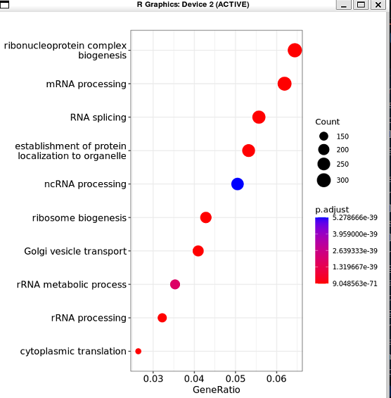
clusterProfiler 包里的一些默认作图方法，例如：

barplot (enrich.go) #富集柱形图
dotplot (enrich.go) #富集气泡图
cnetplot (enrich.go) #网络图展示富集功能和基因的包含关系
emapplot (enrich.go) #网络图展示各富集功能之间共有基因关系
heatplot (enrich.go) #热图展示富集功能和基因的包含关系

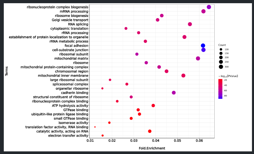
clusterProfiler 包里的图有时候可能不会如我们的愿，于是截取 BP、MF、CC 三个部分的前十个数据，使用 ggplot2 进行绘图 ( 太多会导致很拥挤 ) ：

Term    Fold Enrichment        PValue    Count
ribonucleoprotein complex biogenesis    0.0644         1.43E-74    310
mRNA processing    0.0619         1.19E-58    298
ribosome biogenesis    0.0428         5.89E-56    206
Golgi vesicle transport    0.0409         3.24E-50    197
RNA splicing    0.0557         1.48E-48    268
cytoplasmic translation    0.0264         2.50E-46    127
rRNA processing    0.0322         8.50E-45    155
establishment of protein localization to organelle    0.0532         1.67E-44    256
rRNA metabolic process    0.0353         2.61E-42    170
focal adhesion    0.0617         2.26E-92    304
cell-substrate junction    0.0619         4.74E-89    305

library (dplyr)
library (ggplot2)
library (ggrepel)

GO_data <- read.table ( './data2.txt', header = TRUE,  sep = '\t' )

GO_data <- arrange ( GO_data, GO_data[,3] )

GO_data$Term <- factor ( GO_data$Term, levels = rev ( GO_data$Term ))

mytheme <- theme (
    axis.title = element_text ( face = "bold", size = 14, colour = "black" ) ,
    axis.text = element_text ( face = "bold", size = 14, colour = "black" ) ,
    axis.line = element_line ( size = 0.5, colour = "black" ) ,
    panel.background = element_rect ( colour = "black" ) ,
    legend.key = element_blank ( )
 )

p <- ggplot (
    GO_data,
    aes (
        x = Fold.Enrichment,
        y = Term,
        colour = 1*log10 ( PValue ) ,
        size = Count
 )) +
    geom_point ( ) +
    scale_size ( range = c ( 2,8 )) +
    scale_colour_gradient ( low = "blue", high = "red" ) +
    theme_bw ( ) +
    ylab ( "Terms" ) +
    xlab ( "Fold.Enrichment" ) +
    labs ( color = expression ( -log [10](PValue) ) ) +
    theme ( legend.title = element_text ( margin = margin ( r = 50 )) , axis.title.x = element_text ( margin = margin ( t = 20 )) ) +
    theme ( axis.text.x = element_text ( face = "bold", colour = "black", angle = 0, vjust = 1 ))
plot <- p + mytheme
plot

ggsave ( plot, filename = "GO.png", width = 15, height = 9, dpi = 300 )